SQL Server Architecture – THE LIFE CYCLE OF A QUERY-Part 1

Disclaimer:Hey Guys, this post contains affiliate link to help our reader to buy best product\service for them. It helps us because we receive compensation for our time and expenses.

Lets Begin:-

In this series, we will walk through life cycle of SQL server. Its SQL server 2012 architecture, we have many more new and advanced components introduced and will get introduced in latest version of SQL server. The intention of this blog is to atleast give a basis idea of architecture and SQL query execution.

The Relational and Storage Engines

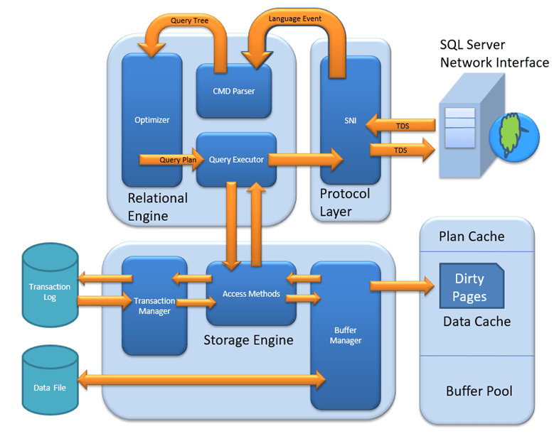
As shown in Figure above, SQL Server is divided into two main engines: the Relational Engine and the Storage Engine. The Relational Engine is also sometimes called the query processor because its primary function is query optimization and execution. It contains a Command Parser to check query syntax and prepare query trees; a Query Optimizer that is arguably the crown jewel of any database system; and a Query Executor responsible for execution.

The Storage Engine is responsible for managing all I/O to the data, and it contains the Access Methods code, which handles I/O requests for rows, indexes, pages, allocations and row versions; and a Buffer Manager, which deals with SQL Server’s main memory consumer, the buffer pool. It also contains a Transaction Manager, which handles the locking of data to maintain isolation (ACID properties) and manages the transaction log.

A Basic SELECT Query

The details of the query used in this example aren’t important — it’s a simple SELECT statement with no joins, so you’re just issuing a basic read request. It begins at the client, where the first component you touch is the SQL Server Network Interface (SNI).

SQL Server Network Interface

The SQL Server Network Interface (SNI) is a protocol layer that establishes the network connection between the client and the server. It consists of a set of APIs that are used by both the database engine and the SQL Server Native Client (SNAC). SNI replaces the net-libraries found in SQL Server 2000 and the Microsoft Data Access Components (MDAC), which are included with Windows.

SNI isn’t configurable directly; you just need to configure a network protocol on the client and the server. SQL Server has support for the following protocols:

Shared memory — Simple and fast, shared memory is the default protocol used to connect from a client running on the same computer as SQL Server. It can only be used locally, has no configurable properties, and is always tried first when connecting from the local machine.
TCP/IP — This is the most commonly used access protocol for SQL Server. It enables you to connect to SQL Server by specifying an IP address and a port number. Typically, this happens automatically when you specify an instance to connect to. Your internal name resolution system resolves the hostname part of the instance name to an IP address, and either you connect to the default TCP port number 1433 for default instances or the SQL Browser service will find the right port for a named instance using UDP port 1434.
Named Pipes — TCP/IP and Named Pipes are comparable protocols in the architectures in which they can be used. Named Pipes was developed for local area networks (LANs) but it can be inefficient across slower networks such as wide area networks (WANs).

To use Named Pipes you first need to enable it in SQL Server Configuration Manager (if you’ll be connecting remotely) and then create a SQL Server alias, which connects to the server using Named Pipes as the protocol.Named Pipes uses TCP port 445, so ensure that the port is open on any firewalls between the two computers, including the Windows Firewall.

VIA — Virtual Interface Adapter is a protocol that enables high-performance communications between two systems. It requires specialized hardware at both ends and a dedicated connection.

Like Named Pipes, to use the VIA protocol you first need to enable it in SQL Server Configuration Manager and then create a SQL Server alias that connects to the server using VIA as the protocol. While SQL Server 2012 still supports the VIA protocol, it will be removed from a future version so new installations using this protocol should be avoided.

Regardless of the network protocol used, once the connection is established, SNI creates a secure connection to a TDS endpoint (described next) on the server, which is then used to send requests and receive data. For the purpose here of following a query through its life cycle, you’re sending the SELECT statement and waiting to receive the result set.

Tabular Data Stream (TDS) Endpoints

TDS is a Microsoft-proprietary protocol originally designed by Sybase that is used to interact with a database server. Once a connection has been made using a network protocol such as TCP/IP, a link is established to the relevant TDS endpoint that then acts as the communication point between the client and the server.

There is one TDS endpoint for each network protocol and an additional one reserved for use by the dedicated administrator connection (DAC). Once connectivity is established, TDS messages are used to communicate between the client and the server.

The SELECT statement is sent to the SQL Server as a TDS message across a TCP/IP connection (TCP/IP is the default protocol).

Protocol Layer

When the protocol layer in SQL Server receives your TDS packet, it has to reverse the work of the SNI at the client and unwrap the packet to find out what request it contains. The protocol layer is also responsible for packaging results and status messages to send back to the client as TDS messages.

Our SELECT statement is marked in the TDS packet as a message of type “SQL Command,” so it’s passed on to the next component, the Query Parser, to begin the path toward execution.

Figure 2 shows where our query has gone so far. At the client, the statement was wrapped in a TDS packet by the SQL Server Network Interface and sent to the protocol layer on the SQL Server where it was unwrapped, identified as a SQL Command, and the code sent to the Command Parser by the SNI.

Command Parser

The Command Parser’s role is to handle T-SQL language events. It first checks the syntax and returns any errors back to the protocol layer to send to the client. If the syntax is valid, then the next step is to generate a query plan or find an existing plan. A query plan contains the details about how SQL Server is going to execute a piece of code. It is commonly referred to as an execution plan.

To check for a query plan, the Command Parser generates a hash of the T-SQL and checks it against the plan cache to determine whether a suitable plan already exists. The plan cache is an area in the buffer pool used to cache query plans. If it finds a match, then the plan is read from cache and passed on to the Query Executor for execution. (The following section explains what happens if it doesn’t find a match.)

1. Plan Cache

Creating execution plans can be time consuming and resource intensive, so it makes sense that if SQL Server has already found a good way to execute a piece of code that it should try to reuse it for subsequent requests.

If no cached plan is found, then the Command Parser generates a query tree based on the T-SQL. A query tree is an internal structure whereby each node in the tree represents an operation in the query that needs to be performed. This tree is then passed to the Query Optimizer to process. Our basic query didn’t have an existing plan so a query tree was created and passed to the Query Optimizer.

Figure 3 shows the plan cache added to the diagram, which is checked by the Command Parser for an existing query plan. Also added is the query tree output from the Command Parser being passed to the optimizer because nothing was found in cache for our query.

Query Optimizer

The Query Optimizer is the most prized possession of the SQL Server team and one of the most complex and secretive parts of the product. Fortunately, it’s only the low-level algorithms and source code that are so well protected (even within Microsoft), and research and observation can reveal how the Optimizer works.

It is what’s known as a “cost-based” optimizer, which means that it evaluates multiple ways to execute a query and then picks the method that it deems will have the lowest cost to execute. This “method” of executing is implemented as a query plan and is the output from the Query Optimizer.

Based on that description, you would be forgiven for thinking that the Optimizer’s job is to find the best query plan because that would seem like an obvious assumption. Its actual job, however, is to find a good plan in a reasonable amount of time, rather than the best plan. The optimizer’s goal is most commonly described as finding the most efficient plan.

If the Optimizer tried to find the “best” plan every time, it might take longer to find the plan than it would to just execute a slower plan (some built-in heuristics actually ensure that it never takes longer to find a good plan than it does to just find a plan and execute it).

As well as being cost based, the Optimizer also performs multi-stage optimization, increasing the number of decisions available to find a good plan at each stage. When a good plan is found, optimization stops at that stage.

The first stage is known as pre-optimization, and queries drop out of the process at this stage when the statement is simple enough that there can only be one optimal plan, removing the need for additional costing. Basic queries with no joins are regarded as “simple,” and plans produced as such have zero cost (because they haven’t been costed) and are referred to as trivial plans.

The next stage is where optimization actually begins, and it consists of three search phases:

Phase 0 — During this phase the optimizer looks at nested loop joins and won’t consider parallel operators .

The optimizer will stop here if the cost of the plan it has found is < 0.2. A plan generated at this phase is known as a transaction processing, or TP, plan.

Phase 1 — Phase 1 uses a subset of the possible optimization rules and looks for common patterns for which it already has a plan.

The optimizer will stop here if the cost of the plan it has found is < 1.0. Plans generated in this phase are called quick plans.

Phase 2 — This final phase is where the optimizer pulls out all the stops and is able to use all of its optimization rules. It also looks at parallelism and indexed views (if you’re running Enterprise Edition).

Completion of Phase 2 is a balance between the cost of the plan found versus the time spent optimizing. Plans created in this phase have an optimization level of “Full.”

HOW MUCH DOES IT COST?

The term cost doesn’t translate into seconds or anything meaningful; it is just an arbitrary number used to assign a value representing the resource cost for a plan. However, its origin was a benchmark on a desktop computer at Microsoft early in SQL Server’s life.In a plan, each operator has a baseline cost, which is then multiplied by the size of the row and the estimated number of rows to get the cost of that operator — and the cost of the plan is the total cost of all the operators.Because cost is created from a baseline value and isn’t related to the speed of your hardware, any plan created will have the same cost on every SQL Server installation (like-for-like version).

Because our SELECT query is very simple, it drops out of the process in the pre-optimization phase because the plan is obvious to the optimizer (a trivial plan). Now that there is a query plan, it’s on to the Query Executor for execution.

Query Executor

The Query Executor’s job is self-explanatory; it executes the query. To be more specific, it executes the query plan by working through each step it contains and interacting with the Storage Engine to retrieve or modify data.NOTEThe interface to the Storage Engine is actually OLE DB, which is a legacy from a design decision made in SQL Server’s history. The development team’s original idea was to interface through OLE DB to allow different Storage Engines to be plugged in. However, the strategy changed soon after that.The idea of a pluggable Storage Engine was dropped and the developers started writing extensions to OLE DB to improve performance. These customizations are now core to the product; and while there’s now no reason to have OLE DB, the existing investment and performance precludes any justification to change it.

The SELECT query needs to retrieve data, so the request is passed to the Storage Engine through an OLE DB interface to the Access Methods.

Access Methods

Access Methods is a collection of code that provides the storage structures for your data and indexes, as well as the interface through which data is retrieved and modified. It contains all the code to retrieve data but it doesn’t actually perform the operation itself; it passes the request to the Buffer Manager.

Suppose our SELECT statement needs to read just a few rows that are all on a single page. The Access Methods code will ask the Buffer Manager to retrieve the page so that it can prepare an OLE DB rowset to pass back to the Relational Engine.

Buffer Manager

The Buffer Manager, as its name suggests, manages the buffer pool, which represents the majority of SQL Server’s memory usage. If you need to read some rows from a page (you’ll look at writes when we look at an UPDATE query), the Buffer Manager checks the data cache in the buffer pool to see if it already has the page cached in memory. If the page is already cached, then the results are passed back to the Access Methods.

If the page isn’t already in cache, then the Buffer Manager gets the page from the database on disk, puts it in the data cache, and passes the results to the Access Methods.

The key point to take away from this is that you only ever work with data in memory. Every new data read that you request is first read from disk and then written to memory (the data cache) before being returned as a result set.

This is why SQL Server needs to maintain a minimum level of free pages in memory; you wouldn’t be able to read any new data if there were no space in cache to put it first.

The Access Methods code determined that the SELECT query needed a single page, so it asked the Buffer Manager to get it. The Buffer Manager checked whether it already had it in the data cache, and then loaded it from disk into the cache when it couldn’t find it.

Data Cache

The data cache is usually the largest part of the buffer pool; therefore, it’s the largest memory consumer within SQL Server. It is here that every data page that is read from disk is written to before being used.

The sys.dm_os_buffer_descriptors DMV contains one row for every data page currently held in cache. You can use this script to see how much space each database is using in the data cache:

SELECT count(*)*8/1024 AS 'Cached Size (MB)'
   ,CASE database_id
        WHEN 32767 THEN 'ResourceDb'
        ELSE db_name(database_id)
        END AS 'Database'
FROM sys.dm_os_buffer_descriptors
GROUP BY db_name(database_id),database_id
ORDER BY 'Cached Size (MB)' DESC

The amount of time that pages stay in cache is determined by a least recently used (LRU) policy.

The header of each page in cache stores details about the last two times it was accessed, and a periodic scan through the cache examines these values. A counter is maintained that is decremented if the page hasn’t been accessed for a while; and when SQL Server needs to free up some cache, the pages with the lowest counter are flushed first.

The process of “aging out” pages from cache and maintaining an available amount of free cache pages for subsequent use can be done by any worker thread after scheduling its own I/O or by the lazy writer process, covered later in the section “Lazy Writer.”

You can view how long SQL Server expects to be able to keep a page in cache by looking at the MSSQL$<instance>:Buffer ManagerPage Life Expectancy counter in Performance Monitor. Page life expectancy (PLE) is the amount of time, in seconds, that SQL Server expects to be able to keep a page in cache.

Under memory pressure, data pages are flushed from cache far more frequently. Microsoft has a long standing recommendation for a minimum of 300 seconds for PLE but a good value is generally considered to be 1000s of seconds these days. Exactly what your acceptable threshold should be is variable depending on your data usage, but more often than not, you’ll find servers with either 1000s of seconds PLE or a lot less than 300, so it’s usually easy to spot a problem.

The database page read to serve the result set for our SELECT query is now in the data cache in the buffer pool and will have an entry in the sys.dm_os_buffer_descriptors DMV. Now that the Buffer Manager has the result set, it’s passed back to the Access Methods to make its way to the client.